This article presents methods of enhancing a wireless link in a typical environment of simple low-power wireless transceivers. It also focuses on maximizing the reliability of a wireless link, while keeping the overall hardware costs down. For many simple transceivers the added overhead of using frequency-hopping diversity hardly seems worthwhile; however, this article presents strong technical reasons why this should be considered even for simple applications.


A wireless channel is a space and frequency dependent, time-variant RF system. This means that the instantaneous performance of the RF channel changes with frequency, time, and physical changes. To obtain a reliable wireless communication link, the wireless system should incorporate techniques that try to use these three vectors to its advantage. For instance, simply changing the frequency of operation is called frequency diversity. Likewise, changing placement in space becomes spatial diversity, and time become time diversity.
Tradeoffs and benefits for each diversity scheme
For each diversity scheme there is an increased system cost in the form of extra hardware or more software complexity. Sometimes there can also be a reduced system capacity because of message repetition. When reviewing the different wireless standards most prevalent today, you will find one or more of them currently in use:
- Space and/or Polarization diversity is used by GSM, DECT and WiFi
a. Extra hardware cost in extra transceivers and antennas
b. Retains full system data rate - Frequency diversity is used by WiFi and Bluetooth
a. No hardware cost, however, extra software complexity applies
b. Reduced total system data rate because of time spent changing frequency - Time diversity (SimpliciTI™)
a. No hardware cost, no significant software complexity
b. Reduced total system data rate by the number of repetitions of data
For systems requiring the highest possible data throughput, enabling spatial diversity often is the correct design path to take [1]. For this article we will focus our attention towards frequency diversity, because it presents the options of adding diversity to a system without adding extra hardware and can, in some cases, still exhibit very low latencies.
Practical measurements on typical low-power wireless links
The following sets of data were taken using a CC2500 development kit. A total of 1000 packets were transmitted. Each packet contains a 64-byte payload and has a trailing cyclic redundancy check (CRC) sum byte. All the measurements are running at 250 Kb/s data rate at a fixed output power of 0 dBm.
Radio channel measurements using a single RF channel at 2.45 GHz
Figure 1 represents data taken over a five-second period, while moving at one-foot-per-second. This data is taken in a residential home with one radio transmitting at 2450 MHz at 0 dBm and one radio receiving the data. The received signal strength indicator (RSSI) and the CRC state is recorded and presented for each burst of data.

Figure 1: Typical indoor non-line-of-sight RSSI performance, while moving at one-foot-per-second (blue). The bottom line (green) represents the returned CRC status. High = CRC valid, Low = CRC error.
In this case, there is no frequency hopping and over 25 dB of variations is found in measured RSSI over a very short time. In some cases it is as short at 2 – 3 bursts (20 – 30ms). This causes a given receiver to miss the incoming data and, therefore, hurt the overall quality of the wireless link. For this particular experiment, 5.3 percent of the incoming packets are either missing or have an invalid CRC check sum.
Characteristics of stationary RF channel over frequency
A very simple version of frequency hopping is implemented where the transmitter increases the frequency of operation after each burst by 1 MHz. For software simplicity reasons, 64 channels were chosen. Running at 1000 bursts gives 15 full sweeps across the 64 MHz frequency band. For frequency hopping schemes, it is very important to calculate the timing budget and allow enough time for the transceiver to change frequency and re-lock its phase-locked loop (PLL). The method of estimating the final burst duration is:
- Burst length calculated at 250 kbits/s in order of transmission
a. 8-byte preample : 0.256 ms
b. 2-byte sync word : 0.064 ms
c. 64-byte payload : 2.048 ms
d. 1-byte CRC sum : 0.032 ms - Change frequency and relock the PLL takes, worst case, 0.9 ms.
Therefore, a total burst time of 3.5 ms should be accounted for. We selected a 10 ms burst window to keep timing requirements simple for this exercise. The results below represent 15 sweeps across the 64 MHz range of operation. The transmitter and receiver are kept stationary for the 10-second duration.
Examine the frequency response from this particular sweep and see how quickly the reported RSSI can drop. In this particular case the reported RSSI value drops from –76 dBm at 2450 MHz to –93 dBm at 2435 MHz. The difference between a good wireless link and a very poor performing link can be a result of a 17 dB change in RSSI. When designing any RF communications systems, it is important to consider this phenomenon and what it will do to your data integrity.
When examining the performance of the RF channel shown in Figure 2, it looks possible to implement a method where the radio characterizes the RF channel and then selects the channels with the best RSSI at which to operate. However, consider a relatively simple case with more than two radios in operation simultaneously. It’s possible that the link between radios one and two is good at a certain frequency, while the link between radios one and three is bad. So, even for some static RF channel use situations, some kind of frequency averaging may be advantageous.

Figure 2: Frequency sweep performance for static indoor non-line-of-sight wireless channel. Fifteen sweeps plotted (thin lines). The thick red line represents an average value of data for each frequency point.
In many cases, it is better to view the performance of a radio channel with respect to time on a contour plot, like that shown in Figure 3, because it shows the behavior of the channel over time. For the static channel, the performance does not change much with time and the results looks like a “river bed” in the vertical direction (which is time).
For dynamic channels the performance changes continuously. Therefore, using avoidance techniques is not possible. To determine this we need to characterize how quickly a RF channel changes when the transmitter (TX) and receiver (RX) are moving.
Characteristics of dynamic RF channel over frequency
A slow moving dynamic channel is characterized using the same frequency hopping RF system as in Figure 3, where a transmitter increases the frequency of operation after each burst by 1 MHz, and using the same total of 1000 bursts.

Figure 3: Reported RSSI value versus frequency (horizontal axis) and time (vertical axis) of a stationary channel. The Y axis represents the frequency sweeps, each taking 640 ms to complete. The X-axis is frequency of operation in MHz, and the color bar on the right translates RSSI values to a color on the graph.
To make the RF channel dynamic, the receiver is moved at a pace of approximately one foot/s inside a residential home. This makes the channel change over time. The results are presented in Figure 4.

Figure 4: Reported RSSI value versus frequency (horizontal axis) and time (vertical axis) of a dynamic channel. The Y axis represents the frequency sweeps, each taking 640 ms to complete. The X-axis is the frequency of operation in MHz and the color bar on the right translates RSSI values to a color on the graph.
In Figure 4, a deep fade moved from 2445 MHz to 2420 MHz over a period of 10 ms. This fade is deep enough to cause the wireless link to not operate at these two frequencies. If a system was operating at only one frequency and that frequency was chosen, the wireless link would be broken.
When looking at this scenario with a little more scrutiny, you can see that for any sweep that is recorded, a large majority of the time the wireless link is operating fine. In this particular case, the system reported three bursts as missing out of a total of 1000 bursts transmitted.
If we could add some kind of encoding scheme to the incoming data stream to enable us to extract the wanted data, even under the influence of burst time errors, we could create a reliable wireless system.
A large number of mathematic procedures are available to perform this encoding and decoding of data[2], and they all revolve around the same basic principle: add redundant data to the incoming data stream. This creates overhead and lowers the overall through-put, but enables the receiver to detect errors and fix them.
Forward error corrections and data interleaving
Encoders are typically separated into two main categories: “block codes” and “convolutional codes." The main difference between the two types of codes is how they operate.
Block codes
The “block code” operates on blocks of data and generates a redundancy code word as a block. The most well-known block code is the “Reed-Solomon code” (RS-code). This code is a subclass of the linear block codes and is widely used in CD/DVD media plus a host of other data storage media[2].
The block code is specified in terms of block length: n=2m-1, where “m” is an integer and the message size “k." The resulting parity check size becomes 2t = (n-k). A typical value for “m” is eight and, therefore, the resulting block length becomes 255 bytes. The size of the parity check is dependent on what levels of data integrity is sought. Be careful to take into account when designing your RS-code the fact that it takes two bytes of parity check to correct one byte of message error.
Convolutional codes
The convolutional coder operates on incoming data in a bit-by-bit sequence, otherwise known as operating in discrete time. The convolutional encoder is used widely by wireless standards, particularly GSM/GPRS. The convolutional code is specified in terms of the constraint length “K” and encoding rate “n." The constraint length “K” defines the number of bits being used to generate a given code word or, in other words, the maximum sequence of bit errors the scheme can handle. The encoding rate “n” gives the relationship between the size of the incoming bits stream and the outbound bit stream. An encoding rate of “n” doubles the number of bits to be transmitted.
Convolutional encoders are computationally very in-expensive to make. The encoder is simple to implement because it consists only of “K” number of shift registers and a number of interconnects with simple module-two adders connecting them in a prescribed fashion. The decoder is a bit more involved but is readily available in various hardware implementations including many modern digital signal processors (DSPs).
Data interleaving
Data interleaving is an important data manipulation function to perform before entering the forward error corrections units described earlier. Especially for convolutional coders with their limited capability to handle multiple consecutive errors, it is important to perform a spreading of the payload encoding it.
Many low-power wireless transceivers have forward error correction with data interleaving in hardware. They work great for single bit errors happening with low-noise situations, but are of little use when faced with fading events large enough to delete an entire burst. For these events, a secondary data interleaver and forward error correction (FEC) should be used across multiple bursts, again looking at GSM/GPRS there, the secondary interleaver works on 8 bursts in parallel.
Frequency hopping schemes
The simplest frequency hopping scheme is a linear one, where the radio simply increases the frequency of operation by a set amount (e.g., 1 MHz) for each time a burst is transmitted. However, from the RF channel characteristics discussed earlier about practical measurements on typical low-power wireless links, you can see that multiple consecutive bursts can be affected by deep fades, if a linear frequency hopping technique is used. The information on forward error corrections and data interleaving shows the forward error corrections techniques, like the convolutional encoders, perform poorly when faced with consecutive errors. Therefore, it is an advantage to implement a system that incorporates a random frequency hopping scheme, which lowers the overall likelihood for consecutive errors.

Figure 5: A linear frequency hopping scheme (left) compared to a pseudo random frequency hopping scheme (right).
Another advantage of using a pseudo random frequency hopping scheme is that it becomes possible to have multiple wireless links running autonomously on top of each other, as long as they use a different random key sequence and incorporate some kind of forward error correction such that they could handle a lost packet due to collisions.
This is one of the features in the frequency hopping scheme used in today’s Bluetooth standard. Whenever two Bluetooth devices are paired, they negotiate which pseudo random frequency hopping key to use and then proceed to use it for all communication going forward. The keys used are different for each connection, which minimizes the chances for sequential collisions.
Conclusions
In this article, we presented three main diversity techniques and we discussed each method’s advantages and system cost. We focused on the option of “no additional hardware cost.” This constraint removes the popular “space diversity” option from consideration. We also gained an understanding of frequency diversity along with time diversity in the form of a simple acknowledge message with retransmissions.
The frequency response of an actual RF channel was characterized using both a fixed frequency setup and a sweeping test setup:
- Fixed – The fixed frequency setup presented fades of approximately 25 dB with these fades lasting between 50 and 200 ms, while moving the transceivers at one foot/s.
- Swept – The swept frequency setup presented drops in reported RSSI of 17 dB over a sub-band of just 15 MHz. While moving the transceivers at one foot/s, the frequency where the fades appeared moved by 25 MHz in 10 ms.
Because of these quick changes in RF channel performance, we can conclude that the best approach for a simple one-antenna RF transceiver would be to include some kind of random frequency hopping scheme to average out the effects of the quickly changing channel performance.
References
- “Low-power wireless devices achieve a reliable wireless link in a multi-path environment,” by Thomas Almholt, RF DesignLine, May 17, 2010.
- “Communication System 3e,” by Simon Haykin: ISBN 0-471-57176-8, (1994).